Comparison between metamixr and RoBMA

This vignette validates the random effects meta analysis and selection model implementation in metamixr against RoBMA. RoBMA priors are set to the metamixr defaults (normal(0, 1) on the mean and half-normal(0, 0.2) on the heterogeneity) so that the two packages estimate the same model. Also see Maier (2026) for a more in depth simulation study validating the mixture models. Reproducing this vignette requires RoBMA (version 4.0.0 or later) and JAGS in addition to package dependencies.

library(metamixr)
library(rstan)
library(RoBMA)

Random-effects meta-analysis

We simulate 300 studies with a true mean effect of 0 and heterogeneity 0.2. We can use the function from the package to specify a normal random effects meta-analysis by setting M = 1 and weights = c(1,1,1) (all studies equally likely to be published).

set.seed(42)
dat <- sim_mix(K = 300, M = 1, mu = 0, tau = 0.2, steps = c(0.95, 0.975),
               weights = c(1, 1, 1), one_sided = TRUE)

The random-effects model in metamixr can be fit using re_mix() with a single component; in RoBMA it can be fitted using brma().

fit_metamix <- re_mix(dat$y, dat$sds, M = 1, chains = 4, cores = 4, seed = 1, refresh = 0)

fit_RoBMA <- brma(yi = dat$y, sei = dat$sds, measure = "GEN",
                  prior_effect = prior("normal", list(0, 1)),
                  prior_heterogeneity = prior("normal", list(0, 0.2), list(0, Inf)),
                  chains = 4, sample = 1000, burnin = 1000, parallel = TRUE, seed = 1)
#> Compiling rjags model...
#> Starting 4 rjags simulations using a PSOCK cluster with 4 nodes on host
#> 'localhost'
#> Simulation complete
#> Finished running the simulation

Both implementations recover the data-generating values and agree closely.

print(fit_metamix, pars = c("mu", "tau"))
#> Inference for Stan model: random_effects_mix.
#> 4 chains, each with iter=2000; warmup=1000; thin=1; 
#> post-warmup draws per chain=1000, total post-warmup draws=4000.
#> 
#>         mean se_mean   sd  2.5%   25%   50%   75% 97.5% n_eff Rhat
#> mu[1]  -0.04       0 0.01 -0.07 -0.05 -0.04 -0.03 -0.01  3397    1
#> tau[1]  0.18       0 0.02  0.15  0.17  0.18  0.19  0.21  3318    1
#> 
#> Samples were drawn using NUTS(diag_e) at Tue Sep 22 12:35:32 2026.
#> For each parameter, n_eff is a crude measure of effective sample size,
#> and Rhat is the potential scale reduction factor on split chains (at 
#> convergence, Rhat=1).
summary(fit_RoBMA)
#> 
#> Bayesian Random-Effects Model (k = 300)
#> 
#> Estimates
#>       Mean    SD  0.025    0.5  0.975 error(MCMC) error(MCMC)/SD  ESS R-hat
#> mu  -0.039 0.016 -0.071 -0.039 -0.008     0.00025          0.016 4000 1.000
#> tau  0.180 0.016  0.149  0.180  0.211     0.00031          0.020 2471 1.001

One-sided selection

Next we simulate publication bias using sim_mix. Studies that are not significant in the expected direction (p > .05 in one-sided test) are published with probability 0.2, marginally significant studies (.025 < p < .05) with probability 0.5, and significant studies with probability 1.

set.seed(123)
dat_pb <- sim_mix(K = 300, M = 1, mu = 0, tau = 0.2, steps = c(0.95, 0.975),
                  weights = c(0.2, 0.5, 1), one_sided = TRUE)

Let’s plot the distribution of z statistics to visually inspect the simulated publciation bias.

z <- dat_pb$y / dat_pb$sds
hist(z, breaks = 60, main = "", xlab = "z-statistic")
abline(v = qnorm(c(0.95, 0.975)), lty = 2)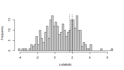

plot of chunk z-hist

The two packages state the same cutoffs differently. metamixr takes cumulative probabilities of the standard normal distribution, steps = c(0.95, 0.975), so that qnorm(steps) are the cutoffs on the z-statistic. RoBMA takes the one-sided p-values, steps = c(0.025, 0.05). To validate the metamixr implementation we restrict RoBMA to fit only a single selection model corresponding to the implementation of the selection model in metamixr.

fit_metamix_pb <- sel_mix(dat_pb$y, dat_pb$sds, M = 1, steps = c(0.95, 0.975),
                          chains = 4, cores = 4, seed = 1, refresh = 0)

fit_RoBMA_pb <- bselmodel(yi = dat_pb$y, sei = dat_pb$sds, measure = "GEN",
                          prior_effect = prior("normal", list(0, 1)),
                          prior_heterogeneity = prior("normal", list(0, 0.2), list(0, Inf)),
                          prior_bias = prior_weightfunction(side = "one-sided",
                                                            steps = c(0.025, 0.05)),
                          effect_direction = "positive",
                          chains = 4, sample = 1000, burnin = 1000, parallel = TRUE, seed = 1)
#> Compiling rjags model...
#> Starting 4 rjags simulations using a PSOCK cluster with 4 nodes on host
#> 'localhost'
#> Simulation complete
#> Finished running the simulation

Again the estimates agree between the two approaches to fitting the same selection model.

print(fit_metamix_pb, pars = c("mu", "tau", "omega"))
#> Inference for Stan model: selection_mix.
#> 4 chains, each with iter=2000; warmup=1000; thin=1; 
#> post-warmup draws per chain=1000, total post-warmup draws=4000.
#> 
#>          mean se_mean   sd  2.5%  25%  50%  75% 97.5% n_eff Rhat
#> mu[1]    0.02       0 0.02 -0.03 0.00 0.02 0.03  0.06  2302    1
#> tau[1]   0.20       0 0.02  0.17 0.19 0.20 0.21  0.23  2174    1
#> omega[1] 0.29       0 0.07  0.18 0.24 0.29 0.34  0.46  2095    1
#> omega[2] 0.57       0 0.15  0.32 0.45 0.55 0.67  0.90  2040    1
#> omega[3] 1.00       0 0.00  1.00 1.00 1.00 1.00  1.00   134    1
#> 
#> Samples were drawn using NUTS(diag_e) at Tue Sep 22 12:38:42 2026.
#> For each parameter, n_eff is a crude measure of effective sample size,
#> and Rhat is the potential scale reduction factor on split chains (at 
#> convergence, Rhat=1).
summary(fit_RoBMA_pb)
#> 
#> Bayesian Random-Effects Selection Model (k = 300)
#> 
#> Estimates
#>      Mean    SD  0.025   0.5 0.975 error(MCMC) error(MCMC)/SD  ESS R-hat
#> mu  0.017 0.024 -0.030 0.017 0.063     0.00096          0.040  729 1.013
#> tau 0.202 0.016  0.171 0.202 0.235     0.00046          0.029 1230 1.003
#> 
#> Publication Bias
#>                    Mean    SD 0.025   0.5 0.975 error(MCMC) error(MCMC)/SD ESS
#> omega[0,0.025]    1.000 0.000 1.000 1.000 1.000          NA             NA  NA
#> omega[0.025,0.05] 0.568 0.147 0.322 0.552 0.891     0.00578          0.039 644
#> omega[0.05,1]     0.293 0.073 0.174 0.284 0.463     0.00313          0.043 599
#>                   R-hat
#> omega[0,0.025]       NA
#> omega[0.025,0.05] 1.010
#> omega[0.05,1]     1.011
#> P-value intervals for publication bias weights omega correspond to one-sided p-values.

Two-sided selection

We next compare the two methods for two sided selection, where significance in either direction increases the probability of publication. In metamixr this is one_sided = FALSE; in RoBMA it is side = "two-sided" in the weight function prior.

set.seed(123)
dat_pb2 <- sim_mix(K = 300, M = 1, mu = 0, tau = 0.2, steps = c(0.95, 0.975),
                   weights = c(0.2, 0.5, 1), one_sided = FALSE)

fit_metamix_pb2 <- sel_mix(dat_pb2$y, dat_pb2$sds, M = 1, steps = c(0.95, 0.975),
                           one_sided = FALSE, chains = 4, cores = 4, seed = 1, refresh = 0)

fit_RoBMA_pb2 <- bselmodel(yi = dat_pb2$y, sei = dat_pb2$sds, measure = "GEN",
                           prior_effect = prior("normal", list(0, 1)),
                           prior_heterogeneity = prior("normal", list(0, 0.2), list(0, Inf)),
                           prior_bias = prior_weightfunction(side = "two-sided",
                                                             steps = c(0.025, 0.05)),
                           chains = 4, sample = 1000, burnin = 1000, parallel = TRUE, seed = 1)
#> Compiling rjags model...
#> Starting 4 rjags simulations using a PSOCK cluster with 4 nodes on host
#> 'localhost'
#> Simulation complete
#> Finished running the simulation

print(fit_metamix_pb2, pars = c("mu", "tau", "omega"))
#> Inference for Stan model: selection_mix.
#> 4 chains, each with iter=2000; warmup=1000; thin=1; 
#> post-warmup draws per chain=1000, total post-warmup draws=4000.
#> 
#>          mean se_mean   sd  2.5%   25%  50%  75% 97.5% n_eff Rhat
#> mu[1]    0.00       0 0.01 -0.03 -0.01 0.00 0.00  0.02  2464    1
#> tau[1]   0.23       0 0.02  0.20  0.22 0.23 0.24  0.26  2930    1
#> omega[1] 0.31       0 0.06  0.22  0.27 0.31 0.35  0.43  3086    1
#> omega[2] 0.50       0 0.11  0.31  0.42 0.49 0.57  0.75  2093    1
#> omega[3] 1.00       0 0.00  1.00  1.00 1.00 1.00  1.00   256    1
#> 
#> Samples were drawn using NUTS(diag_e) at Tue Sep 22 12:44:07 2026.
#> For each parameter, n_eff is a crude measure of effective sample size,
#> and Rhat is the potential scale reduction factor on split chains (at 
#> convergence, Rhat=1).
summary(fit_RoBMA_pb2)
#> 
#> Bayesian Random-Effects Selection Model (k = 300)
#> 
#> Estimates
#>       Mean    SD  0.025    0.5 0.975 error(MCMC) error(MCMC)/SD  ESS R-hat
#> mu  -0.004 0.014 -0.031 -0.004 0.023     0.00029          0.021 2245 1.002
#> tau  0.227 0.018  0.193  0.226 0.262     0.00060          0.034  874 1.001
#> 
#> Publication Bias
#>                    Mean    SD 0.025   0.5 0.975 error(MCMC) error(MCMC)/SD  ESS
#> omega[0,0.025]    1.000 0.000 1.000 1.000 1.000          NA             NA   NA
#> omega[0.025,0.05] 0.871 0.095 0.651 0.891 0.995     0.00296          0.031 1022
#> omega[0.05,1]     0.315 0.057 0.217 0.310 0.440     0.00185          0.033  944
#>                   R-hat
#> omega[0,0.025]       NA
#> omega[0.025,0.05] 1.008
#> omega[0.05,1]     1.002
#> P-value intervals for publication bias weights omega correspond to one-sided p-values.

References

Bartoš, F., Maier, M., Wagenmakers, E.-J., Doucouliagos, H., & Stanley, T. D. (2023). Robust Bayesian meta-analysis: Model-averaging across complementary publication bias adjustment methods. Research Synthesis Methods, 14(1), 99–116. https://doi.org/10.1002/jrsm.1594

Maier, M. (2026). Addressing heterogeneity with Bayesian meta-analytic mixture modelling. PsyArXiv. https://doi.org/10.31234/osf.io/nkyqm_v2

Maier, M., Bartoš, F., & Wagenmakers, E.-J. (2023). Robust Bayesian meta-analysis: Addressing publication bias with model-averaging. Psychological Methods, 28(1), 107–122. https://doi.org/10.1037/met0000405

Maximilian Maier

Random-effects meta-analysis

One-sided selection

Two-sided selection

References